Ch02: More in Excel 2019

CHAPTER 2 - More in Excel 2019

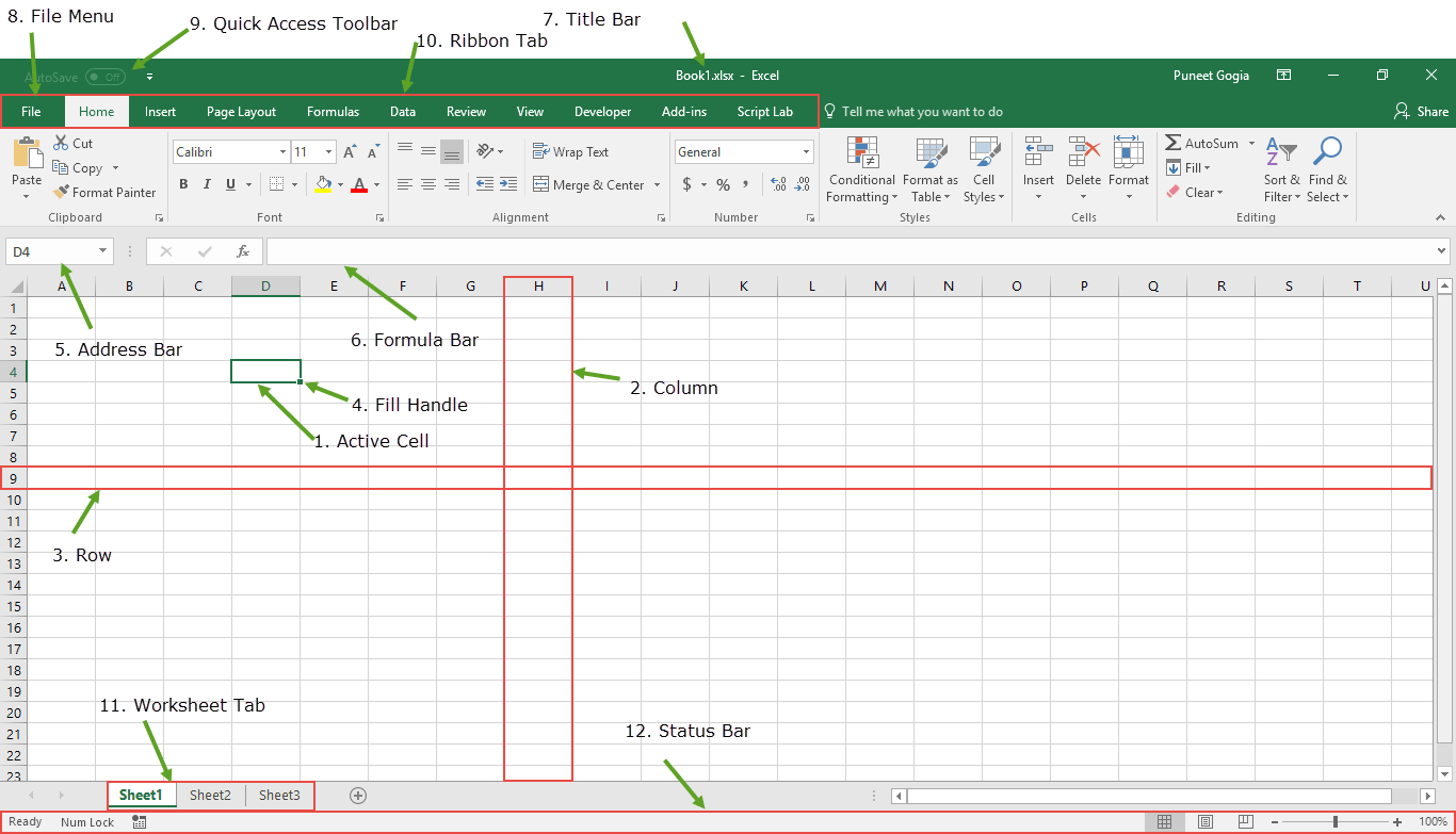
📘 Introduction to Excel 2019

Microsoft Excel is a spreadsheet program used to:

• Store data in rows and columns
• Perform calculations
• Create charts and graphs
• Sort and filter data
• Analyze large amounts of information

Excel is widely used in schools, offices, banks, and businesses.

1️⃣ SUM() Function

Meaning: Used to add numbers quickly.

Syntax:

=SUM(number1, number2, ...)

=SUM(A1:A5)

Example:

A
10
20
30

=SUM(A1:A3)

Result = 60

Steps:

1. Select any cell
2. Type =SUM(A1:A3)
3. Press Enter

2️⃣ IF() Function

Meaning: Checks condition and gives different results.

Syntax:

=IF(condition, true_result, false_result)

Example:

Formula: =IF(A1>=40,"Pass","Fail")

If marks are 50 → Pass

If marks are 30 → Fail

Marks	Result
50	Pass
30	Fail

Uses:

1. Result sheet
2. Salary bonus
3. Attendance check

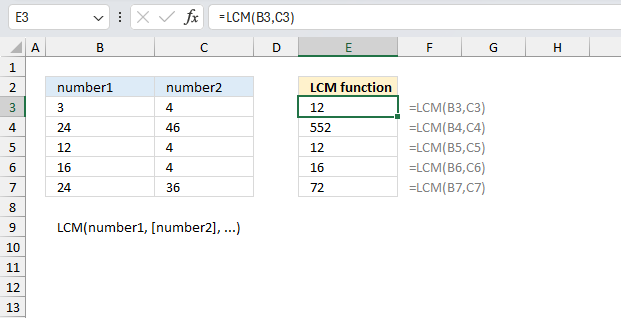
3️⃣ LCM() Function

Finds Least Common Multiple.

Gives smallest common multiple of numbers.

=LCM(4,6)

Result = 12

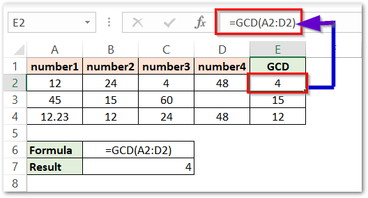
4️⃣ GCD() Function

Finds Greatest Common Divisor.

Formula: =GCD(12,18)

Answer: 6

5️⃣ Data Sorting

Meaning: Arranging data in order.

• Ascending Order (A-Z / Small-Large)
• Descending Order (Z-A / Large-Small)

Example:

Before Sorting: Ram, Aman, Riya

After Sorting: Aman, Ram, Riya

Steps:

1. Select data
2. Click Data Tab
3. Choose Sort A-Z or Z-A

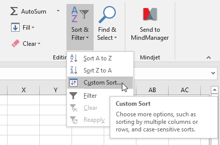
6️⃣ Custom Sorting

Meaning: Sorting by multiple columns.

Example: Sort by Class, Name, Marks

1. Select table
2. Click Data Tab
3. Click Sort
4. Add levels

7️⃣ Filtering Data

Meaning: Show only selected records.

Example: Students above 80 marks.

1. Select heading row
2. Data Tab
3. Click Filter

Dropdown arrows appear.

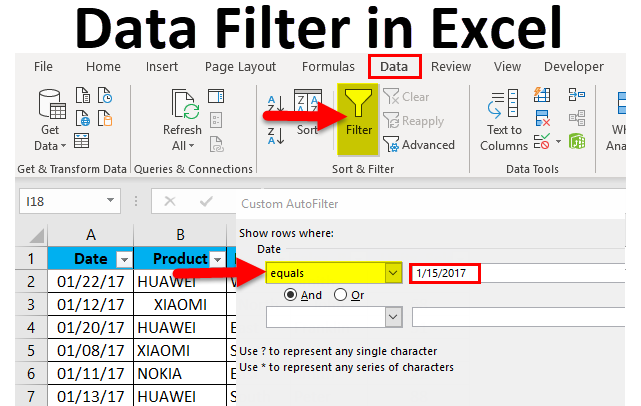
8️⃣ Custom Filters

Meaning: Used for special conditions.

• Greater than 50
• Less than 100
• Begins with A

Example: Marks > 70

9️⃣ Removing Filters

Meaning: Show all data again.

1. Go to Data Tab
2. Click Filter again
3. Choose Clear Filter

🔟 Conditional Formatting

Meaning: Highlight cells automatically.

• Red color for low marks
• Green for high marks
• Duplicate values highlight

Steps:

1. Select cells
2. Home Tab
3. Conditional Formatting
4. Choose rule

Example: Marks below 40 become red.

MS Excel Chapter Exercise Solution

A. Tick (✔) the Correct Option

1. Which function checks whether a condition is true or false?
✔ (c) IF()

2. The Sort & Filter option is present under ______ group.
✔ (d) Both (a) & (b)

3. Which key combination is used to filter the data?
✔ (b) Ctrl + Shift + L

4. Conditional formatting allows us to ______
✔ (a) Change the appearance of a cell

5. Which function is the largest positive integer that divides numbers without remainder?
✔ (c) HCF()

B. Fill in the Blanks

1. The SUM() function adds all the numbers given in the range of cells.
2. IF() is used when you need to test more than one values.
3. The LCM is the smallest positive integer.
4. When we arrange data in ascending or descending order, it is called Sorting.
5. Excel also allows you to use Functions.
6. Conditional Formatting allows you to change the appearance of a cell.

C. True / False

Statement	Answer
1. In MS Excel, functions are predefined operations.	✔ True
2. LCM() function returns the least common multiple of integers.	✔ True
3. Filtering offers a quick way to analyze data.	✔ True
4. We cannot apply conditional formatting in Excel worksheet.	✘ False
5. Sorting option is present under Data tab.	✔ True

D. Answer the Following Questions

1. What is the use of SUM function? How can we use this function?
Answer: The SUM() function is used to add numbers quickly in Excel. It saves time and gives accurate results.
Example: =SUM(A1:A5) adds all numbers from cell A1 to A5.

2. What do you know about IF function?
Answer: The IF() function is used to check a condition. If the condition is true, it gives one result, and if false, it gives another result.
Example: =IF(A1>=50,"Pass","Fail")

3. What do you understand by filtering data in MS Excel?
Answer: Filtering means displaying only the required data and hiding unnecessary data. It helps to analyze information easily and quickly.

4. What is Data Sorting? Write the steps to use data sorting.
Answer: Data Sorting means arranging data in a specific order such as ascending or descending.

Steps to Sort Data:

• Select the data range.
• Click on the Data tab.
• Choose Sort A to Z or Sort Z to A.
• Your data will be arranged automatically.

5. Define Conditional Formatting. How can we apply conditional formatting?
Answer: Conditional Formatting is a feature used to change the appearance of cells according to given conditions. It highlights important data using colors, icons, or bars.

Steps to Apply Conditional Formatting:

• Select the cells.
• Click the Home tab.
• Choose Conditional Formatting.
• Select any rule or style.
• The selected formatting will be applied.